The Futility of Buying the Dip
Background
This is an analysis I did in 2016 to convince myself that buying the dip is smart. At that point, I had two years of savings but not invested anything in the stock market because I thought that it was overpriced and that I would be better off sitting it out and going in after the inevitable big crash. Ironically, this analysis convinced me not to try to buy the dip and I ended up investing everything I had immediately after.
Assumptions
I made some very strong simplifying assumptions. You should feel free to skip this post if they seem too naive to you. I considered them reasonable given the level of effort, risk and sophistication that I desired, but they certainly don’t make sense for everyone.
- I only looked at stocks, specifically the S&P500, as a proxy for an investment portfolio.
- I ignored dividends and only considered capital gains.
- I assumed that we don’t use financial derivatives.
- I assumed a pure buy-and-hold strategy. We don’t have to think about selling, only when to buy and how much.
Strategies
The naive way to study buying the dip would be to test out different ways of predicting dips. However, there are infinite techniques for making these predictions. So even if one strategy doesn’t work, it doesn’t negate the class of strategies.
We can overcome this by reframing the problem: Forget about the individual strategies. Let’s just test the perfect strategy against the naive strategy and see how they compare.
The perfect strategy is quite simply knowing the future, which we can model with the benefit of hindsight. At any point in time, the perfect strategy given knowledge of some period in future is to check if there is a lower price in sight. If so, keep saving for that upcoming dip. If not, we’re at the bottom of any foreseeable dip so buy as much as possible. Remember that this is only optimal because we never sell and because we’re ignoring dividends, so holding stock doesn’t accrue any other benefits beyond capital appreciation.
One the other end of the spectrum is the naive strategy that has absolutely no foresight. If we have no idea about the future except that stock appreciates in the long run, the best we can do is to buy as much as possible right now.
In this analysis, I tested strategies with zero (naive), one, ten, hundred and thousand business days of foresight.
Results
The astounding thing is that the thousand day strategy only saw a 14.6% increase in net worth after 35 years (1980-2016). A thousand business days is roughly 4 years. The improbability of picking out the right day in a 4 year period, and the intestinal fortitude needed to sit on 2 years (expected value) of savings and go all in on that one fateful day, makes this 14.6% payoff seem measly.
| Strategy | Net Worth (MM) | Cash | Stock | Net Worth Increase (%) | |
|---|---|---|---|---|---|
| 0 | greedy | 21.13 | 0.0016 | 9931.73 | 0.00 |
| 1 | one_day | 21.28 | 0.001068 | 9999.64 | 0.68 |
| 2 | ten_day | 21.69 | 0.0007 | 10192.14 | 2.62 |
| 3 | hundred_day | 22.85 | 0.0006 | 10736.65 | 8.10 |
| 4 | thousand_day | 24.23 | 0.0012 | 11388.07 | 14.66 |
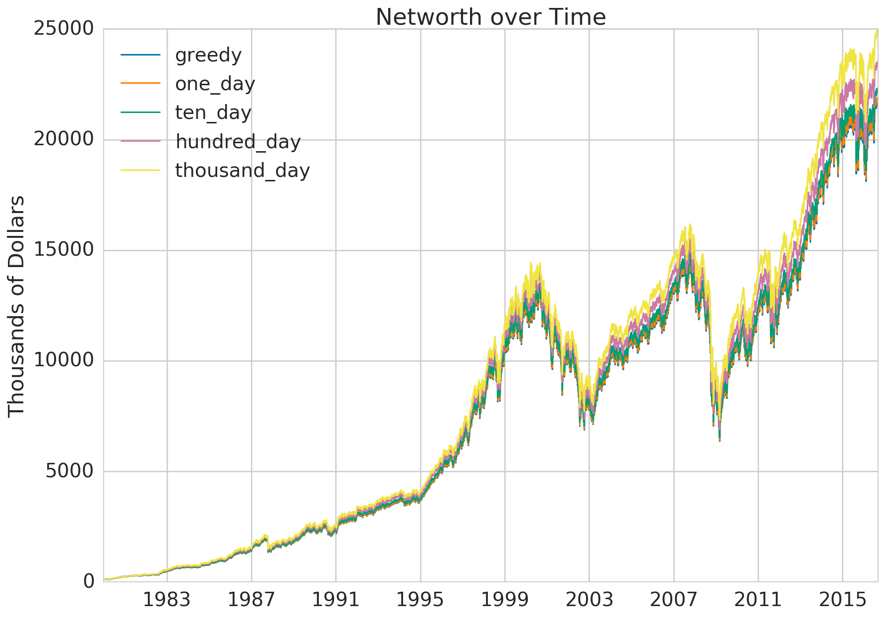
The graph below shows the net worth of the strategies over time. Observe how closely they follow each other. The boom and bust cycles appear to be more than 4 years long, so perhaps we would need five thousand days of foresight to see a significant advantage.
The next graph gives us a perspective of the underlying stock purchasing behavior of the strategies. In the lead-up to the dotcom crash, between 1998 and 2002, the thousand day buy-the-dip strategy was able to hoard cash. It didn’t purchase any stock during that time and only went in heavily when the market was at its lowest. The same thing happened between 2004 and 2008 in the lead-up to the the great financial crisis.
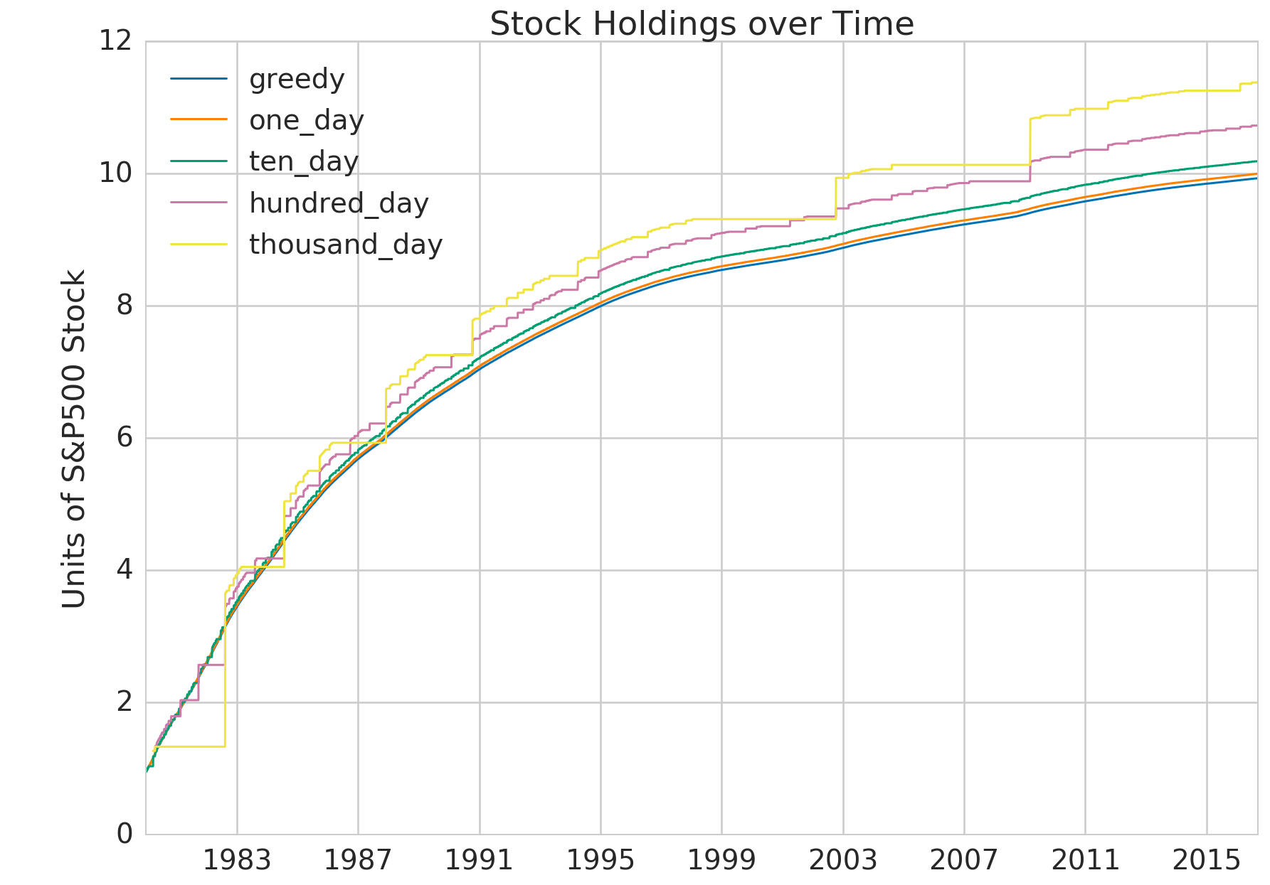
No doubt these episodes allowed the buy-the-dip strategies to come out ahead. However, the graph shows that for long stretches of time (1983 to 1998 and 2008 to 2016), the buy-the-dip strategies, even with all their unnatural foresight, still found it optimal to slowly accumulate stock. It was during these long periods of incremental growth that all strategies built up significant portions of their net worth, eventually dwarfing gains from the periods of hoarding. This is why buy-the-dip strategies were only marginally better, especially given all the work that they require.
The Grunt Work
The data analysis was quite straightforward. Here’s the code in case you want to play around with it.
1. Preparing Data
I obtained daily historical data of the S&P 500 from Yahoo Finance and did some basic preparation of the data. You can download it here.
df = pd.read_csv('yahoo_s&p500_historical.csv')
df['Date'] = pd.to_datetime(df['Date'])

# Yahoo Finance data in reverse chronological order.
# Start from the future, use 'rolling' to work backwards to find the dips.
df['One Day Low'] = df['Close'].rolling(1+1, min_periods=1).min()
df['Ten Day Low'] = df['Close'].rolling(1+10, min_periods=1).min()
df['Hundred Day Low'] = df['Close'].rolling(1+100, min_periods=1).min()
df['Thousand Day Low'] = df['Close'].rolling(1+1000, min_periods=1).min()

# Sort the entries in chronological order so we can iterate through them later.
df.sort_values('Date', inplace=True)
df.tail()
| Date | Open | High | Low | Close | Volume | Adj Close | One Day Low | Ten Day Low | Hundred Day Low | Thousand Day Low | |
|---|---|---|---|---|---|---|---|---|---|---|---|
| 4 | 2016-09-02 | 2177.489990 | 2184.870117 | 2173.590088 | 2179.979980 | 3091120000 | 2179.979980 | 2179.979980 | 2127.810059 | 2127.810059 | 2127.810059 |
| 3 | 2016-09-06 | 2181.610107 | 2186.570068 | 2175.100098 | 2186.479980 | 3447650000 | 2186.479980 | 2186.159912 | 2127.810059 | 2127.810059 | 2127.810059 |
| 2 | 2016-09-07 | 2185.169922 | 2187.870117 | 2179.070068 | 2186.159912 | 3319420000 | 2186.159912 | 2181.300049 | 2127.810059 | 2127.810059 | 2127.810059 |
| 1 | 2016-09-08 | 2182.760010 | 2184.939941 | 2177.489990 | 2181.300049 | 3727840000 | 2181.300049 | 2127.810059 | 2127.810059 | 2127.810059 | 2127.810059 |
| 0 | 2016-09-09 | 2169.080078 | 2169.080078 | 2127.810059 | 2127.810059 | 4233960000 | 2127.810059 | 2127.810059 | 2127.810059 | 2127.810059 | 2127.810059 |
2. Account Abstraction
This is a simple abstraction for modeling my investment account. It serves a few basic functions:
- Tracks current holdings of stock and cash. (
self.cur_hdg) - Records historical net worth, ie. the total dollar value of all holdings on each day. (
self.hist_networth) - Adds interest payments on the cash held. (
earn_interest()) - Implements a function for buying stock that limits expediture based on current cash holdings. (
budget_buy())
import collections
ANNUAL_BUSINESS_DAYS = 250
class Account:
    def __init__(self, start_hdg, annual_interest=0.01):
        self.start_hdg = start_hdg
        self.cur_hdg = collections.OrderedDict(start_hdg)
        if 'cash' not in self.cur_hdg:
            self.cur_hdg['cash'] = 0.0

        self.annual_interest = annual_interest

        self.hist_networth = []

    def _buy(self, asset, amt, unit_price):
        total_expenditure = amt * unit_price
        assert total_expenditure <= self.cur_hdg['cash'], 'not enough cash'
        self.cur_hdg['cash'] -= total_expenditure
        self.cur_hdg[asset] = self.cur_hdg.get(asset, 0) + amt

    def budget_buy(self, asset, amt, unit_price):
        # prevent going over budget due to rounding errors
        amt = np.floor(amt * 1e6) / 1e6
        total_expenditure = amt * unit_price
        if total_expenditure > self.cur_hdg['cash']:
            vetted_amt = self.cur_hdg['cash'] / unit_price
        else:
            vetted_amt = amt
        self._buy(asset, vetted_amt, unit_price)
        return vetted_amt * unit_price

    def update_networth(self, date, cur_asset_prices):
        cur_asset_prices['cash'] = 1.0
        networth = sum(amt * cur_asset_prices[asset]
                       for asset, amt in self.cur_hdg.items())
        self.hist_networth.append([date, networth] + list(self.cur_hdg.values()))

    def earn_interest(self, interest):
        self.cur_hdg['cash'] *= (1.0 + interest)

    def process_day(self, date, cur_asset_prices, daily_interest=True):
        if daily_interest:
            self.earn_interest(self.annual_interest / ANNUAL_BUSINESS_DAYS)
        self.update_networth(date, cur_asset_prices)
3. Run Models
I created five investment accounts, each starting with $100K, earning $100K annually, and having its own investment strategy. As mentioned before, the greedy model bought as much stock as it could, as soon as it could. The other four were buy-the-dip strategies with the ability to pick dips by looking 1, 10, 100 and 1000 days into the future.
accounts = []
accounts.append({'name': 'greedy', 'account': Account({'cash': 100000}), 'low_column': 'Close'})
accounts.append({'name': 'one_day', 'account': Account({'cash': 100000}), 'low_column': 'One Day Low'})
accounts.append({'name': 'ten_day', 'account': Account({'cash': 100000}), 'low_column': 'Ten Day Low'})
accounts.append({'name': 'hundred_day', 'account': Account({'cash': 100000}), 'low_column': 'Hundred Day Low'})
accounts.append({'name': 'thousand_day', 'account': Account({'cash': 100000}), 'low_column': 'Thousand Day Low'})
data_range = df[df.Date > pd.to_datetime('1980-01-01')]
daily_salary = 100000.0 / ANNUAL_BUSINESS_DAYS
I iterated through the days in the time period, having each account earn salary, make buying decisions based on respective strategy and record net worth.
for _, row in data_range.iterrows():
    for account in accounts:
        account_object = account['account']
        account_object.cur_hdg['cash'] += daily_salary

        # Check the low for the given lookahead period.
        # If that low occurs today, buy with what you have. Otherwise, wait.
        if row['Close'] <= row[account['low_column']]:
            account_object.budget_buy('s&p', account_object.cur_hdg['cash'] / row.Close, row.Close)

        account_object.process_day(row.Date, {'s&p': row['Close']})
Now we just have to extract the data stored in our account objects.
final_results = []
for account in accounts:
    account_df = pd.DataFrame(account['account'].hist_networth, columns=['Date', 'Networth', 'cash', 's&p'])
    account.update({'account_df': account_df})
    final_row = account_df.iloc[-1,:]
    final_results.append({'Net Worth (MM)': final_row['Networth']/1e6,
                          'Cash': final_row['cash'],
                          'Stock': final_row['s&p'],
                          'Strategy':account['name']})
4. Plot Results
final_df = pd.DataFrame(final_results)[['Strategy', 'Net Worth (MM)', 'Cash', 'Stock']]
greedy_networth = final_df[final_df['Strategy']=='greedy']['Net Worth (MM)'][0]
final_df['Net Worth Increase (%)'] = 100 * (final_df['Net Worth (MM)']/greedy_networth - 1)
final_df
# Displays the table above
for account in accounts:
    df = account['account_df']
    plt.plot(df['Date'], df['Networth']/1e3, label=account['name'], linewidth=1.5)
plt.legend(loc='upper left')
plt.ylabel('Thousands of Dollars')
plt.title('Networth over Time')
# Displays the net worth graph above
for account in accounts:
    df = account['account_df']
    plt.plot(df['Date'], df['s&p']/1e3, label=account['name'], linewidth=1.5)
plt.legend(loc='upper left')
plt.ylabel('Units of S&P500 Stock')
plt.title('Stock Holdings over Time')
# Displays the stock holdings graph above